


Turingは、効果的なベイズ推論と意思決定のための、汎用の確率プログラミング言語です。モデル記述の可読性が高く、処理が高速です。経済、その他、社会学分野の分析に使う場合でも、モデルの作成が容易です。この分野ではよく知られているRichard McElreathのStatisticalRethinkingが参考になります。StatisticalRethinkingはRとStanで記述されていますが、この内容をjuliaにポートしたチュートリアルが以下のGitで利用可能です。
https://github.com/StatisticalRethinkingJulia/TuringModels.jl
特徴
- 確率プログラムは、@modelマクロでラップされるjuliaのコードです。
- 推論メソッドとして、Importance sampling(IS), シーケンシャルモンテカルロ(SMC),パーティクルギッブス(PG),ハミルトニアンモンテカルロ(HMC),デュアルアベレージング・ハミルトニアン・モンテカルロ(HMCDA),No-U-Turnサンプラー(NUTS)を提供します。
- サンプリングの間、バックエンドで四種類の自動微分のパッケージをサポートしています。Forward-mode AD, 3種類のリバースモードAD,Tracker,Zygote,ReverseDiffです。バックエンドの自動微分は切り替えて使用することができます。
- サンプラーとしてDynamicHMCパッケージが使えます
HMCを最適化したDynamicHMCは、以下のGit、および参考資料を参照してください。
https://github.com/tpapp/DynamicHMC.jl
参考資料:DynamicHMCの解説.
- Betancourt, M. J., Byrne, S., & Girolami, M. (2014). Optimizing the integrator step size for Hamiltonian Monte Carlo. arXiv preprint arXiv:1411.6669.
- Betancourt, M. (2017). A Conceptual Introduction to Hamiltonian Monte Carlo. arXiv preprint arXiv:1701.02434.
- TArray データ型を使います。
- Turingプログラムは、ランダム変数のために
~表記を使います。x~distrこれは、distr分布に従うランダム変数xを宣言します。前述のStatistical Rethinkingにおけるモデルの記述と同じシンタックスでソースコードが記述できます。
推論を実行するには、sample関数を使います。サンプラーの種類は、上に記した推論メソッドに一致します。
c1 = sample(gdemo(1.5, 2), SMC(), 1000)
c2 = sample(gdemo(1.5, 2), PG(10), 1000)
c3 = sample(gdemo(1.5, 2), HMC(0.1, 5), 1000)
c4 = sample(gdemo(1.5, 2), Gibbs(PG(10, :m), HMC(0.1, 5, :s²)), 1000)
c5 = sample(gdemo(1.5, 2), HMCDA(0.15, 0.65), 1000)
c6 = sample(gdemo(1.5, 2), NUTS(0.65), 1000)
sample関数の第一引数は、モデルの定義です。以下の例にあるように@modelマクロを使って定義します。
using Turing
using StatsPlots

# 未知の平均と分散を持つガウシアンモデルを定義
@model function gdemo(x, y)
    s² ~ InverseGamma(2, 3)
    m ~ Normal(0, sqrt(s²))
    x ~ Normal(m, sqrt(s²))
    y ~ Normal(m, sqrt(s²))
end
サンプラーの出力結果をまとめて出力します。以下は、上記モデルをHMCでサンプリングしたc3(ハミルトニアンモンテカルロ)の出力です。
# 結果
describe(c3)

# 出力
plot(c3)
参考文献
Richard McElreath. Statistical Rethinking. A Bayesian Course with Examples in R and Stan.
Turingのインストール
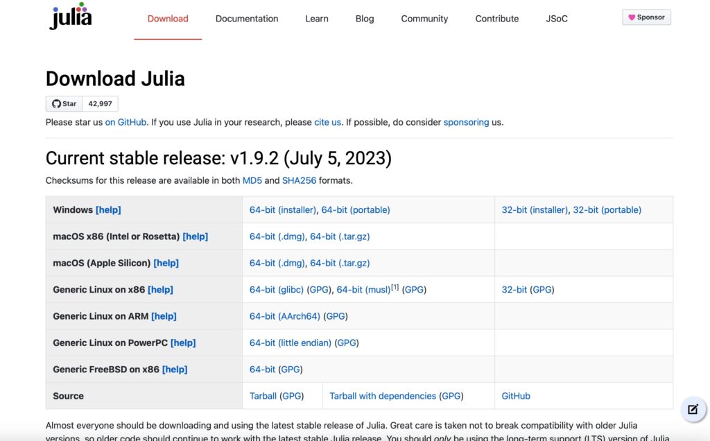
Turingはjuliaのライブラリです。juliaのインストールは以下のWebsiteから、Host環境に応じて最新のバージョンをダウンロードします。
Juliaの環境変数の設定などは、以下の記事を参照してください。

Turingのインストールは、juliaのREPLから以下のコマンドを実行します。
julia> ]
(@v1.9) pkg> add Turing
(@v1.9) pkg> add Turing
Updating registry at `~/.julia/registries/General.toml`
Resolving package versions...
Installed AbstractMCMC ─────────────── v4.4.2
Installed AxisArrays ───────────────── v0.4.7
Installed NaturalSort ──────────────── v1.0.0
Installed LRUCache ─────────────────── v1.4.1
Installed StatisticalTraits ────────── v3.2.0
Installed ConsoleProgressMonitor ───── v0.1.2
Installed FFTW ─────────────────────── v1.7.1
Installed AdvancedPS ───────────────── v0.4.3
Installed Turing ───────────────────── v0.29.0
Installed ProgressMeter ────────────── v1.8.0
Installed Optimisers ───────────────── v0.2.20
Installed Roots ────────────────────── v2.0.19
Installed IntelOpenMP_jll ──────────── v2023.2.0+0
Installed EnumX ────────────────────── v1.0.4
Installed RandomNumbers ────────────── v1.5.3
Installed ZygoteRules ──────────────── v0.2.3
Installed RecursiveArrayTools ──────── v2.38.7
Installed LogDensityProblemsAD ─────── v1.6.1
Installed EllipticalSliceSampling ──── v1.1.0
Installed Tricks ───────────────────── v0.1.7
Installed RealDot ──────────────────── v0.1.0
Installed SimpleUnPack ─────────────── v1.1.0
Installed ADTypes ──────────────────── v0.1.6
Installed Bijectors ────────────────── v0.13.7
Installed ProgressLogging ──────────── v0.1.4
Installed Functors ─────────────────── v0.4.5
Installed SciMLBase ────────────────── v1.96.2
Installed DynamicPPL ───────────────── v0.23.16
Installed Ratios ───────────────────── v0.4.5
Installed MCMCDiagnosticTools ──────── v0.3.5
Installed Random123 ────────────────── v1.6.1
Installed LeftChildRightSiblingTrees ─ v0.2.0
Installed ExprTools ────────────────── v0.1.10
Installed ChainRules ───────────────── v1.54.0
Installed Lazy ─────────────────────── v0.15.1
Installed Tracker ──────────────────── v0.2.26
Installed MCMCChains ───────────────── v6.0.3
...以下のコマンドで、Turing APIの各機能をテストできます。テストする場合は、所要時間として1時間以上要します。
(@v1.9) pkg> test Turing(@v1.9) pkg> test Turing
Testing Turing
Status `/private/var/folders/z3/y2vb_4653kjcytsygg5bkv7w0000gn/T/jl_AVRILo/Project.toml`
[80f14c24] AbstractMCMC v4.4.2
[5b7e9947] AdvancedMH v0.7.5
[576499cb] AdvancedPS v0.4.3
[b5ca4192] AdvancedVI v0.2.4
.....テスト結果の表示です。
Test Summary: | Pass  Total      Time
Turing        | 1668   1668  96m33.9s
 ────────────────────────────────────────────────────────────────────────────
                                                  Time          Allocations
                                            ───────────────   ───────────────
               Total measured:                   1.61h             593GiB

 Section                            ncalls     time    %tot     alloc    %tot
 ────────────────────────────────────────────────────────────────────────────
 essential/ad.jl                         1     163s    2.8%   40.1GiB    6.8%
 mcmc/particle_mcmc.jl                   1    22.5s    0.4%   5.16GiB    0.9%
 mcmc/emcee.jl                           1    13.2s    0.2%   5.88GiB    1.0%
 mcmc/ess.jl                             1     427s    7.4%   47.9GiB    8.1%
 mcmc/is.jl                              1    2.61s    0.0%    866MiB    0.1%
 inference: forwarddiff                  1    2383s   41.1%    247GiB   41.6%
   mcmc/gibbs.jl                         1     897s   15.5%   70.7GiB   11.9%
   mcmc/gibbs_conditional.jl             1    22.7s    0.4%   7.46GiB    1.3%
   mcmc/hmc.jl                           1     182s    3.1%   16.9GiB    2.9%
   mcmc/Inference.jl                     1     981s   16.9%   56.9GiB    9.6%
   mcmc/sghmc.jl                         1    4.16s    0.1%   1.26GiB    0.2%
   mcmc/abstractmcmc.jl                  1     140s    2.4%   54.9GiB    9.3%
   mcmc/mh.jl                            1    43.2s    0.7%   9.77GiB    1.6%
   ext/dynamichmc.jl                     1    6.83s    0.1%   1.60GiB    0.3%
   variational/advi.jl                   1    24.0s    0.4%   7.41GiB    1.2%
   optimisation/OptimInterface.jl        1    64.5s    1.1%   15.9GiB    2.7%
   ext/Optimisation.jl                   1    16.9s    0.3%   3.73GiB    0.6%
 inference: reversediff                  1    2598s   44.8%    195GiB   32.9%
   mcmc/gibbs.jl                         1    1037s   17.9%   69.5GiB   11.7%
   mcmc/gibbs_conditional.jl             1    22.0s    0.4%   7.81GiB    1.3%
   mcmc/hmc.jl                           1     306s    5.3%   14.7GiB    2.5%
   mcmc/Inference.jl                     1    1118s   19.3%   51.2GiB    8.6%
   mcmc/sghmc.jl                         1    4.36s    0.1%   1.45GiB    0.2%
   mcmc/abstractmcmc.jl                  1    59.0s    1.0%   36.1GiB    6.1%
   mcmc/mh.jl                            1    27.7s    0.5%   6.67GiB    1.1%
   ext/dynamichmc.jl                     1    2.24s    0.0%    935MiB    0.2%
   variational/advi.jl                   1    16.6s    0.3%   5.91GiB    1.0%
   optimisation/OptimInterface.jl        1    4.65s    0.1%    939MiB    0.2%
   ext/Optimisation.jl                   1    198ms    0.0%   5.30MiB    0.0%
 variational/optimisers.jl               1    4.42s    0.1%   5.01GiB    0.8%
 stdlib/distributions.jl                 1     118s    2.0%   34.1GiB    5.7%
 stdlib/RandomMeasures.jl                1    9.36s    0.2%   1.63GiB    0.3%
 mcmc/utilities.jl                       1    52.3s    0.9%   10.7GiB    1.8%
 ────────────────────────────────────────────────────────────────────────────     Testing Turing tests passed

(@v1.9) pkg>
以下の例で、実際にTuringを使ってみましょう。
例1:ガウシアン回帰
using Turing
using StatsPlots

# Define a simple Normal model with unknown mean and variance.
@model function gdemo(x, y)
  s² ~ InverseGamma(2, 3)
  m ~ Normal(0, sqrt(s²))
  x ~ Normal(m, sqrt(s²))
  y ~ Normal(m, sqrt(s²))
end

#  Run sampler, collect results
chn = sample(gdemo(1.5, 2), HMC(0.1, 5), 1000)

# Summarise results
describe(chn)

# Plot and save results
p = plot(chn)
ライブラリを読み込んで、ガウシアンモデルを定義します。
julia> @model function gdemo(x, y)
         s² ~ InverseGamma(2, 3)
         m ~ Normal(0, sqrt(s²))
         x ~ Normal(m, sqrt(s²))
         y ~ Normal(m, sqrt(s²))
       end
gdemo (generic function with 2 methods)HMCでサンプラーを起動します。
julia> chn = sample(gdemo(1.5, 2), HMC(0.1, 5), 1000)Sampling 100%|██████████████████████████████████████████| Time: 0:00:03
Chains MCMC chain (1000×12×1 Array{Float64, 3}):
Iterations = 1:1:1000
Number of chains = 1
Samples per chain = 1000
Wall duration = 3.66 seconds
Compute duration = 3.66 seconds
parameters = s², m
internals = lp, n_steps, is_accept, acceptance_rate, log_density, hamiltonian_energy, hamiltonian_energy_error, numerical_error, step_size, nom_step_size
Summary Statistics
parameters mean std mcse ess_bulk ess_tail rhat e ⋯
Symbol Float64 Float64 Float64 Float64 Float64 Float64 ⋯
s² 1.9883 1.2989 0.1000 168.7413 319.5199 1.0032 ⋯
m 1.2743 0.8206 0.0837 98.9222 105.0415 1.0306 ⋯
1 column omitted
Quantiles
parameters 2.5% 25.0% 50.0% 75.0% 97.5%
Symbol Float64 Float64 Float64 Float64 Float64
s² 0.6374 1.1334 1.6324 2.4269 5.6600
m -0.3066 0.7265 1.2705 1.7933 2.9907
サンプル結果をまとめます。
julia> describe(chn)2-element Vector{ChainDataFrame}:
Summary Statistics (2 x 8)
Quantiles (2 x 6)結果を表示します。
julia> p = plot(chn)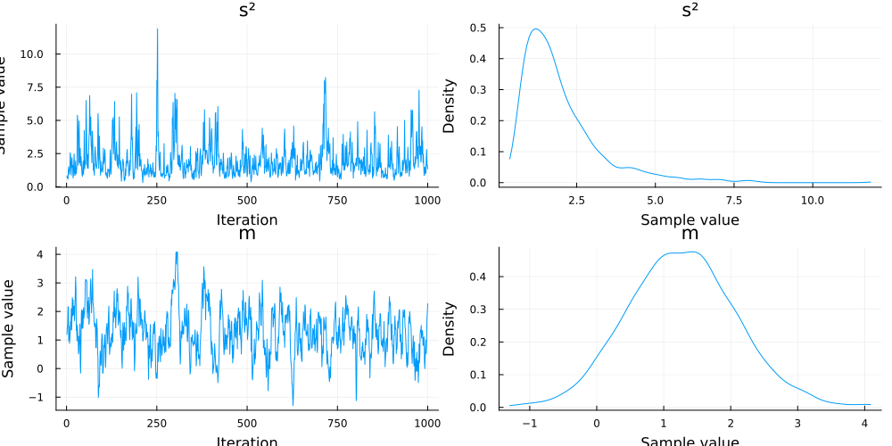
例2:ベイジアン・ニューラルネットワーク
もうひとつ、ベイジアンニューラルネットを例に取り上げます。
ニューラルネットの構築には、juliaの機械学習用ライブラリ、fluxを使用します。fluxはCUDA環境とともに、NVIDIA GPUをサポートします。AMD GPUにはAMD GPUパッケージ、AppleSilicon用にはMetalパッケージをインストールしてください。
以下のコマンドで、FluxでGPUが利用できるか確認できます。NVIDIAの場合、
julia> using CUDA

julia> CUDA.functional()
MACで使用しているAppleSiliconでは、以下のコマンドを使います。
julia> using Metal
julia> Metal.functional()trueAppleSiliconに内蔵のGPUが利用できます。
該当ライブラリがインストールされていない場合、インストールしてください。
julia> using Metal
 │ Package Metal not found, but a package named Metal is available from a
 │ registry.
 │ Install package?
 │   (@v1.9) pkg> add Metal
 └ (y/n/o) [y]: y
   Resolving package versions...
   Installed Metal_LLVM_Tools_jll ─ v0.5.1+0
   Installed Python_jll ─────────── v3.10.8+1
   Installed LoggingExtras ──────── v1.0.2
   Installed Unitful ────────────── v1.17.0
   Installed StatsAPI ───────────── v1.7.0
   Installed LLVMExtra_jll ──────── v0.0.25+0
......
以下はjuliaのソースコードです。
In this tutorial, we demonstrate how one can implement a Bayesian Neural Network using a combination of Turing and [Flux](https://github.com/FluxML/Flux.jl), a suite of machine learning tools. We will use Flux to specify the neural network's layers and Turing to implement the probabilistic inference, with the goal of implementing a classification algorithm.
We will begin with importing the relevant libraries.
```julia
using Turing
using FillArrays
using Flux
using Plots
using ReverseDiff
using LinearAlgebra
using Random
# Use reverse_diff due to the number of parameters in neural networks.
Turing.setadbackend(:reversediff)
```
Our goal here is to use a Bayesian neural network to classify points in an artificial dataset.
The code below generates data points arranged in a box-like pattern and displays a graph of the dataset we will be working with.
```julia
# Number of points to generate.
N = 80
M = round(Int, N / 4)
Random.seed!(1234)
# Generate artificial data.
x1s = rand(M) * 4.5;
x2s = rand(M) * 4.5;
xt1s = Array([[x1s[i] + 0.5; x2s[i] + 0.5] for i in 1:M])
x1s = rand(M) * 4.5;
x2s = rand(M) * 4.5;
append!(xt1s, Array([[x1s[i] - 5; x2s[i] - 5] for i in 1:M]))
x1s = rand(M) * 4.5;
x2s = rand(M) * 4.5;
xt0s = Array([[x1s[i] + 0.5; x2s[i] - 5] for i in 1:M])
x1s = rand(M) * 4.5;
x2s = rand(M) * 4.5;
append!(xt0s, Array([[x1s[i] - 5; x2s[i] + 0.5] for i in 1:M]))
# Store all the data for later.
xs = [xt1s; xt0s]
ts = [ones(2 * M); zeros(2 * M)]
# Plot data points.
function plot_data()
x1 = map(e -> e[1], xt1s)
y1 = map(e -> e[2], xt1s)
x2 = map(e -> e[1], xt0s)
y2 = map(e -> e[2], xt0s)
Plots.scatter(x1, y1; color="red", clim=(0, 1))
return Plots.scatter!(x2, y2; color="blue", clim=(0, 1))
end
plot_data()
```
## Building a Neural Network
The next step is to define a [feedforward neural network](https://en.wikipedia.org/wiki/Feedforward_neural_network) where we express our parameters as distributions, and not single points as with traditional neural networks.
For this we will use `Dense` to define liner layers and compose them via `Chain`, both are neural network primitives from Flux.
The network `nn_initial` we created has two hidden layers with `tanh` activations and one output layer with sigmoid (`σ`) activation, as shown below.
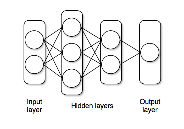
The `nn_initial` is an instance that acts as a function and can take data as inputs and output predictions.
We will define distributions on the neural network parameters and use `destructure` from Flux to extract the parameters as `parameters_initial`.
The function `destructure` also returns another function `reconstruct` that can take (new) parameters in and return us a neural network instance whose architecture is the same as `nn_initial` but with updated parameters.
```julia
# Construct a neural network using Flux
nn_initial = Chain(Dense(2, 3, tanh), Dense(3, 2, tanh), Dense(2, 1, σ))
# Extract weights and a helper function to reconstruct NN from weights
parameters_initial, reconstruct = Flux.destructure(nn_initial)
length(parameters_initial) # number of paraemters in NN
```
The probabilistic model specification below creates a `parameters` variable, which has IID normal variables. The `parameters` vector represents all parameters of our neural net (weights and biases).
```julia
@model function bayes_nn(xs, ts, nparameters, reconstruct; alpha=0.09)
# Create the weight and bias vector.
parameters ~ MvNormal(Zeros(nparameters), I / alpha)
# Construct NN from parameters
nn = reconstruct(parameters)
# Forward NN to make predictions
preds = nn(xs)
# Observe each prediction.
for i in 1:length(ts)
ts[i] ~ Bernoulli(preds[i])
end
end;
```
Inference can now be performed by calling `sample`. We use the `NUTS` Hamiltonian Monte Carlo sampler here.
```julia
# Perform inference.
N = 5000
ch = sample(bayes_nn(hcat(xs...), ts, length(parameters_initial), reconstruct), NUTS(), N);
```
Now we extract the parameter samples from the sampled chain as `theta` (this is of size `5000 x 20` where `5000` is the number of iterations and `20` is the number of parameters).
We'll use these primarily to determine how good our model's classifier is.
```julia
# Extract all weight and bias parameters.
theta = MCMCChains.group(ch, :parameters).value;
```
## Prediction Visualization
We can use [MAP estimation](https://en.wikipedia.org/wiki/Maximum_a_posteriori_estimation) to classify our population by using the set of weights that provided the highest log posterior.
```julia
# A helper to create NN from weights `theta` and run it through data `x`
nn_forward(x, theta) = reconstruct(theta)(x)
# Plot the data we have.
plot_data()
# Find the index that provided the highest log posterior in the chain.
_, i = findmax(ch[:lp])
# Extract the max row value from i.
i = i.I[1]
# Plot the posterior distribution with a contour plot
x1_range = collect(range(-6; stop=6, length=25))
x2_range = collect(range(-6; stop=6, length=25))
Z = [nn_forward([x1, x2], theta[i, :])[1] for x1 in x1_range, x2 in x2_range]
contour!(x1_range, x2_range, Z)
```
The contour plot above shows that the MAP method is not too bad at classifying our data.
Now we can visualize our predictions.
$$
p(\tilde{x} | X, \alpha) = \int_{\theta} p(\tilde{x} | \theta) p(\theta | X, \alpha) \approx \sum_{\theta \sim p(\theta | X, \alpha)}f_{\theta}(\tilde{x})
$$
The `nn_predict` function takes the average predicted value from a network parameterized by weights drawn from the MCMC chain.
```julia
# Return the average predicted value across
# multiple weights.
function nn_predict(x, theta, num)
return mean([nn_forward(x, theta[i, :])[1] for i in 1:10:num])
end;
```
Next, we use the `nn_predict` function to predict the value at a sample of points where the `x1` and `x2` coordinates range between -6 and 6. As we can see below, we still have a satisfactory fit to our data, and more importantly, we can also see where the neural network is uncertain about its predictions much easier---those regions between cluster boundaries.
```julia
# Plot the average prediction.
plot_data()
n_end = 1500
x1_range = collect(range(-6; stop=6, length=25))
x2_range = collect(range(-6; stop=6, length=25))
Z = [nn_predict([x1, x2], theta, n_end)[1] for x1 in x1_range, x2 in x2_range]
contour!(x1_range, x2_range, Z)
```
Suppose we are interested in how the predictive power of our Bayesian neural network evolved between samples. In that case, the following graph displays an animation of the contour plot generated from the network weights in samples 1 to 1,000.
```julia
# Number of iterations to plot.
n_end = 500
anim = @gif for i in 1:n_end
plot_data()
Z = [nn_forward([x1, x2], theta[i, :])[1] for x1 in x1_range, x2 in x2_range]
contour!(x1_range, x2_range, Z; title="Iteration $i", clim=(0, 1))
end every 5
```
This has been an introduction to the applications of Turing and Flux in defining Bayesian neural networks.
```julia, echo=false, skip="notebook", tangle=false
if isdefined(Main, :TuringTutorials)
Main.TuringTutorials.tutorial_footer(WEAVE_ARGS[:folder], WEAVE_ARGS[:file])
end
```サンプラーのバックエンドの自動微分には、RiverseDiffを使います。
julia> Turing.setadbackend(:reversediff):reversediffjulia> N = 80
80
julia> M = round(Int, N / 4)
20
julia> Random.seed!(1234)
TaskLocalRNG()
julia> x1s = rand(M) * 4.5;
julia> x2s = rand(M) * 4.5;
julia> xt1s = Array([[x1s[i] + 0.5; x2s[i] + 0.5] for i in 1:M])20-element Vector{Vector{Float64}}:
[3.109379540603596, 0.875480402444553]
[2.3508235307743273, 2.8660804874110517]
[4.874612371049609, 4.282884137652053]
[0.5670898217829498, 2.8577652727245093]
[2.8415974717567307, 0.5578072545751506]
[3.37802719856123, 2.3257863901499993]
[4.27829870326132, 1.0583352450200438]
[4.852142460119223, 3.4199321922178614]
[4.053939842908088, 4.615882255173184]
[3.632183141647551, 2.0010322726601935]
[3.0501693614468754, 2.0659794637895343]
[2.913658559281987, 2.8791233374992875]
[3.70125162201719, 4.812483426868058]
[0.9676825721140361, 0.5964834515897361]
[4.130168520624449, 2.1317298496814825]
[4.417427025034329, 0.5140448124042801]
[1.0896154529938658, 1.1060839880613769]
[4.7590395180412255, 2.893546052301156]
[3.0844556837524286, 0.8292691129393175]
[3.5494245841981007, 2.7579019034906835]julia> x1s = rand(M) * 4.5;
julia> x2s = rand(M) * 4.5;
julia> append!(xt1s, Array([[x1s[i] - 5; x2s[i] - 5] for i in 1:M]))40-element Vector{Vector{Float64}}:
[3.109379540603596, 0.875480402444553]
[2.3508235307743273, 2.8660804874110517]
[4.874612371049609, 4.282884137652053]
[0.5670898217829498, 2.8577652727245093]
[2.8415974717567307, 0.5578072545751506]
[3.37802719856123, 2.3257863901499993]
[4.27829870326132, 1.0583352450200438]
[4.852142460119223, 3.4199321922178614]
[4.053939842908088, 4.615882255173184]
[3.632183141647551, 2.0010322726601935]
⋮
[-2.5096374764096216, -4.750373512501421]
[-3.964233526461936, -4.759860033104974]
[-4.554470604802372, -2.3881885272694285]
[-4.051993015963654, -3.1268576990325907]
[-4.882145139757624, -4.296324213437888]
[-4.108556974522879, -3.173328328582441]
[-1.80878864973088, -3.0802230410190363]
[-2.3688296784945946, -3.599967464525765]
[-4.159932986770457, -1.0269079318604581]julia> x1s = rand(M) * 4.5;
julia> x2s = rand(M) * 4.5;
julia> xt0s = Array([[x1s[i] + 0.5; x2s[i] - 5] for i in 1:M])20-element Vector{Vector{Float64}}:
[2.467888521928556, -3.0353111818198126]
[4.385204858116833, -2.1077927859071353]
[3.945727337587673, -2.263297388204036]
[4.162178973580089, -2.7500327809867695]
[3.4106592555235085, -2.655964186119601]
[2.095597866949623, -2.742171345884853]
[3.101179141603849, -4.681755779838541]
[1.6939326816288773, -4.718613523852467]
[4.945998712393232, -4.306582117185519]
[1.9763015689773997, -1.1675094920701365]
[1.9451937561727677, -1.311697256378599]
[0.9882093425941452, -1.4452415317022158]
[1.1378737502132756, -4.646419877533919]
[4.568862856781345, -4.324809936393679]
[2.3760330349547525, -2.818285016621949]
[4.976645789195104, -4.133940516167866]
[2.7091996177031255, -2.1493924196077314]
[4.243819766703901, -3.6728215586918553]
[4.512421869396656, -3.809075103911253]
[0.9486134745419225, -1.9173298880509524]
julia> x1s = rand(M) * 4.5;
julia> x2s = rand(M) * 4.5;
julia> append!(xt0s, Array([[x1s[i] - 5; x2s[i] + 0.5] for i in 1:M]))
40-element Vector{Vector{Float64}}:
[2.467888521928556, -3.0353111818198126]
[4.385204858116833, -2.1077927859071353]
[3.945727337587673, -2.263297388204036]
[4.162178973580089, -2.7500327809867695]
[3.4106592555235085, -2.655964186119601]
[2.095597866949623, -2.742171345884853]
[3.101179141603849, -4.681755779838541]
[1.6939326816288773, -4.718613523852467]
[4.945998712393232, -4.306582117185519]
[1.9763015689773997, -1.1675094920701365]
⋮
[-4.042815584290964, 2.9727748685480915]
[-2.3252530557988, 3.7415362522733786]
[-1.4878494145482857, 3.4732450374381223]
[-4.523657835334698, 2.5439676633918418]
[-1.5101252703918089, 0.8623033476433755]
[-1.136545526294888, 3.90015119206306]
[-3.249595279718828, 1.1236114678368896]
[-1.4289842504525416, 3.1096680409747006]
[-4.151060038815406, 4.597779592733514]julia> xs = [xt1s; xt0s]80-element Vector{Vector{Float64}}:
[3.109379540603596, 0.875480402444553]
[2.3508235307743273, 2.8660804874110517]
[4.874612371049609, 4.282884137652053]
[0.5670898217829498, 2.8577652727245093]
[2.8415974717567307, 0.5578072545751506]
[3.37802719856123, 2.3257863901499993]
[4.27829870326132, 1.0583352450200438]
[4.852142460119223, 3.4199321922178614]
[4.053939842908088, 4.615882255173184]
[3.632183141647551, 2.0010322726601935]
⋮
[-4.042815584290964, 2.9727748685480915]
[-2.3252530557988, 3.7415362522733786]
[-1.4878494145482857, 3.4732450374381223]
[-4.523657835334698, 2.5439676633918418]
[-1.5101252703918089, 0.8623033476433755]
[-1.136545526294888, 3.90015119206306]
[-3.249595279718828, 1.1236114678368896]
[-1.4289842504525416, 3.1096680409747006]
[-4.151060038815406, 4.597779592733514]julia> ts = [ones(2 * M); zeros(2 * M)]80-element Vector{Float64}:
1.0
1.0
1.0
1.0
1.0
1.0
1.0
1.0
1.0
1.0
⋮
0.0
0.0
0.0
0.0
0.0
0.0
0.0
0.0
0.0julia> function plot_data() x1 = map(e -> e[1], xt1s)
y1 = map(e -> e[2], xt1s)
x2 = map(e -> e[1], xt0s)
y2 = map(e -> e[2], xt0s)
Plots.scatter(x1, y1; color="red", clim=(0, 1))
return Plots.scatter!(x2, y2; color="blue", clim=(0, 1))
end
plot_data (generic function with 1 method)julia> plot_data()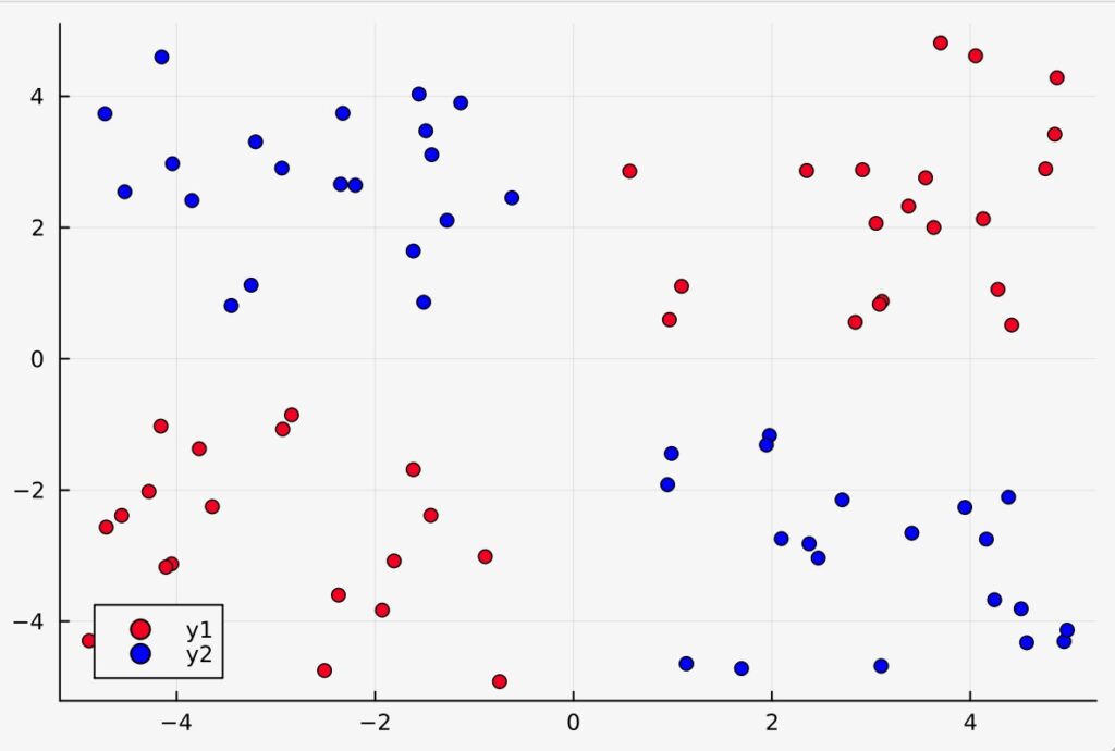
Fluxを使って、ニューラルネットワークを構築します。
julia> nn_initial = Chain(Dense(2, 3, tanh), Dense(3, 2, tanh), Dense(2, 1, σ))
Chain(
  Dense(2 => 3, tanh),                  # 9 parameters
  Dense(3 => 2, tanh),                  # 8 parameters
  Dense(2 => 1, σ),                     # 3 parameters
)                   # Total: 6 arrays, 20 parameters, 464 bytes.
julia> parameters_initial, reconstruct = Flux.destructure(nn_initial)(Float32[0.45902184, -0.061040785, 0.10210564, 0.7931934, 0.8064206, -0.08225103, 0.0, 0.0, 0.0, -1.041428, -0.2038429, -0.061772726, 0.3354218, 0.21408159, -0.27859768, 0.0, 0.0, -0.8626716, 0.47074372, 0.0], Restructure(Chain, ..., 20))julia> length(parameters_initial)20Turingを使った確率モデルでパラメータ変数を作ります。
@model function bayes_nn(xs, ts, nparameters, reconstruct; alpha=0.09)
    # Create the weight and bias vector.
    parameters ~ MvNormal(Zeros(nparameters), I / alpha)

    # Construct NN from parameters
    nn = reconstruct(parameters)
    # Forward NN to make predictions
    preds = nn(xs)

    # Observe each prediction.
    for i in 1:length(ts)
        ts[i] ~ Bernoulli(preds[i])
    end
end;
推論のためにサンプラーを起動します。
julia> N = 5000
julia> ch = sample(bayes_nn(hcat(xs...), ts, length(parameters_initial), reconstruct), NUTS(), N);
┌ Info: Found initial step size
└ ϵ = 0.4
Sampling 100%|██████████████████████████████████████████| Time: 0:16:31julia> theta = MCMCChains.group(ch, :parameters).value;
julia> nn_forward(x, theta) = reconstruct(theta)(x)plot_data()julia> _, i = findmax(ch[:lp])
(-49.626132849706515, CartesianIndex(2151, 1))i = i.I[1]2151x1_range = collect(range(-6; stop=6, length=25))25-element Vector{Float64}:
-6.0
-5.5
-5.0
-4.5
-4.0
-3.5
-3.0
-2.5
-2.0
-1.5
⋮
2.0
2.5
3.0
3.5
4.0
4.5
5.0
5.5
6.0x2_range = collect(range(-6; stop=6, length=25))25-element Vector{Float64}:
-6.0
-5.5
-5.0
-4.5
-4.0
-3.5
-3.0
-2.5
-2.0
-1.5
⋮
2.0
2.5
3.0
3.5
4.0
4.5
5.0
5.5
6.0julia> Z = [nn_forward([x1, x2], theta[i, :])[1] for x1 in x1_range, x2 in x2_range]25×25 Matrix{Float32}:
0.994155 0.994155 0.994155 … 0.0105499 0.01055 0.01055
0.994155 0.994155 0.994155 0.0105499 0.01055 0.01055
0.994155 0.994155 0.994155 0.01055 0.0105501 0.0105501
0.994155 0.994155 0.994155 0.0105502 0.0105504 0.0105505
0.994155 0.994155 0.994155 0.0105511 0.0105516 0.0105523
0.994155 0.994155 0.994155 … 0.0105544 0.0105566 0.0105597
0.994155 0.994155 0.994155 0.0105688 0.0105778 0.0105912
0.994155 0.994155 0.994155 0.0106317 0.0106732 0.0107379
0.994154 0.994154 0.994153 0.010954 0.0112074 0.0116682
0.99415 0.994148 0.994145 0.0137849 0.0174187 0.0274219
⋮ ⋱
0.00951358 0.00923108 0.00914509 0.990554 0.990557 0.99056
0.0091064 0.00909996 0.00909685 0.990562 0.990563 0.990564
0.0090945 0.00909385 0.00909345 0.990564 0.990564 0.990564
0.00909307 0.00909295 0.00909286 0.990565 0.990565 0.990565
0.00909278 0.00909275 0.00909274 … 0.990565 0.990565 0.990565
0.00909271 0.00909271 0.00909269 0.990565 0.990565 0.990565
0.00909269 0.00909269 0.00909269 0.990565 0.990565 0.990565
0.0090927 0.0090927 0.0090927 0.990565 0.990565 0.990565
0.0090927 0.0090927 0.0090927 0.990565 0.990565 0.990565julia> contour!(x1_range, x2_range, Z)julia> function nn_predict(x, theta, num)
return mean([nn_forward(x, theta[i, :])[1] for i in 1:10:num])
end;julia> plot_data()julia> n_end = 1500
1500
julia> x1_range = collect(range(-6; stop=6, length=25))25-element Vector{Float64}:
-6.0
-5.5
-5.0
-4.5
-4.0
-3.5
-3.0
-2.5
-2.0
-1.5
⋮
2.0
2.5
3.0
3.5
4.0
4.5
5.0
5.5
6.0julia> x2_range = collect(range(-6; stop=6, length=25))25-element Vector{Float64}:
-6.0
-5.5
-5.0
-4.5
-4.0
-3.5
-3.0
-2.5
-2.0
-1.5
⋮
2.0
2.5
3.0
3.5
4.0
4.5
5.0
5.5
6.0julia> Z = [nn_predict([x1, x2], theta, n_end)[1] for x1 in x1_range, x2 in x2_range]25×25 Matrix{Float32}:
0.976724 0.976042 0.976017 … 0.0216148 0.0215769 0.0215556
0.976711 0.976729 0.976301 0.0213343 0.021195 0.0212478
0.976699 0.976715 0.976734 0.0209423 0.020966 0.0209183
0.976696 0.9767 0.97672 0.0204603 0.0205138 0.0208422
0.976694 0.976695 0.976701 0.0198328 0.0201531 0.0202904
0.976682 0.976686 0.976691 … 0.0190468 0.0191633 0.019353
0.976682 0.976652 0.976658 0.0183736 0.0184878 0.0190302
0.974535 0.976613 0.976618 0.0182049 0.018569 0.0255911
0.97222 0.972646 0.97533 0.0187005 0.0260868 0.033108
0.966196 0.97163 0.972136 0.0311763 0.0488323 0.0708078
⋮ ⋱
0.0689344 0.0370827 0.0238859 0.963855 0.949968 0.949758
0.0370552 0.0229802 0.0213626 0.968849 0.964801 0.953223
0.0231118 0.021959 0.0206964 0.96882 0.968821 0.965837
0.0223855 0.0211831 0.020024 0.9649 0.968789 0.968804
0.0216957 0.0202223 0.019083 … 0.968684 0.965035 0.965297
0.0206613 0.0192062 0.01815 0.968723 0.96873 0.968683
0.0233717 0.018393 0.0169739 0.968723 0.968724 0.968734
0.0247437 0.0220147 0.017092 0.968725 0.968724 0.968724
0.0234669 0.0233242 0.0225477 0.96873 0.968725 0.968724julia> contour!(x1_range, x2_range, Z)n_end = 500
anim = @gif for i in 1:n_end
plot_data()
Z = [nn_forward([x1, x2], theta[i, :])[1] for x1 in x1_range, x2 in x2_range]
contour!(x1_range, x2_range, Z; title="Iteration $i", clim=(0, 1))
end every 5