グラフィカル・モデルを基にした因果探索

Rによるベイジアンネットワークを用いた因果探索。

有向グラフ因果モデル(DGCMs)、またはDAGは、因果関係を説明し、データから真の因果の関係を探索するために計算に用いる方法です。

causal-learnやcausalpyというpythonの因果探索ライブラリを評価しました、Rにも同様のライブラリが提供されています。ここでは、CRANに登録されているRのライブラリpcalgとbnlearnに実装されているいくつかの因果探索アルゴリズムを評価します。

: causal-learnによる因果探索
　【マネーサプライと物価上昇の因果推論】で、二つの時系列データ間のGranger因果性を調べました。ベクター自己回帰モデル(Vector Auto-Regression:VAR)を適用したものです。他 ...

: 為替レートと地政学的リスク- 割り込まれた時系列データのCausalPyによる分析
　R版の因果推論パッケージCausalImpactの評価のために、軍事侵攻が外国為替レートに与えた影響を、counterfactual推論(注1)の例として紹介しました。このCausalImpactの ...

２０２５年の１０大リスク

　ユーラシア・グループは、毎年、その年の地政学リスクを発表しています。

　2025年は以下のリスクを挙げています。

G0の世界の混迷、 (The G-Zero Wins)
トランプの支配、(Rule of DON)
米中決裂、 (US-CHINA Breakdown)
トランプノミクス、 (Trumponomics)
ならずもの国家のロシア、(Russia Still Rogue)
追い詰められたイラン、(Iran on the Ropes)
世界経済への負の押し付け、 (Beggar thy world)
制御不能なAI、 (AI unbound)
統治なく領域の拡大、 (Ungoverned Spaces)
米国とメキシコの対立、(Mexican Standoff)

　ユーラシアの視点では、第二期トランプ政権の影響が強く反映されています。合衆国のリベラリズムから保護主義的な政策への大きな転換は、グローバル経済に対する影響として多くの国が認識しています。ユーラシアは１０大リスクの背後にある要因として現代が、1930年代や冷戦初期のように危険な時代に入りつつあると指摘しています¹。

　このリストは象徴的なので、ユーラシア・グループが発表している今年の１０大リスクをリスクファクターにして、市場への影響(market fluctuation)を調査するための擬似データとして生成しアルゴリズムを評価します。

　本来、このような使い方はしませんが、グラフィカル・モデルを使う因果探索ツール(Rのライブラリ)の評価用に、現実の観測データとは無関係の合成データを作ります。

　評価するアルゴリズムは、pc(Perter-Clark), FCI, FCI+, Bayesian Network, MMHC, Hill-Climbing, HITON-PC。これらのアルゴリズムを用いてデータから因果関係を探索し、結果をDAGで示します。

　因果の探索の目的は、これらのリスク要因と市場の変動の因果関係を識別することです。

パッケージのインストール

　以下のライブラリを使用します。

library(pcalg)
library(bnlearn)
library(igraph)

　install.packages()コマンドを使って、Rのパッケージをインストールしてください。

install.packages("pcalg")

　graphライブラリが不足して、インストールに失敗する場合があります。

　Rの最新バージョン4.4.2(2025年1月時点)で、graphライブラリのインストールに問題が発生した場合、以下に示すコマンドを実行してください。

　graphライブラリは、現在CRANレポジトリに登録されていません。Bioconductorのホームページからロードするようになっています。

　インストールの方法は、R 4.4 を走らせて、コマンドラインから以下のコマンドを実行してください。

if (!require("BioManager", quietly=TRUE))
　　　　install.packages("BiocManager")
BiocManager::install("graph")

　もう一つの方法として、以下のBioconductorのホームページから、ローカルフォルダにファイルをダウンロードしてインストールすることができます。その場合、以下のページからロードし、ローカルファイルからインストールします。

http://www.bioconductor.org/packages/release/bioc/html/graph.html

install.packages("yourpath/graph_1.56.0.zip",repos=NULL)

　また、同様にRBGL,RgraphvizもCRANレポジトリから削除されています。これらのパッケージがインストールされていない場合、以下のコマンドでインストールしてください。

if (!require("BiocManager", quietly = TRUE))
    install.packages("BiocManager")

BiocManager::install("RBGL")

　Rgraphviz パッケージがインストールされていない場合、

 if (!require("BiocManager", quietly = TRUE))
    install.packages("BiocManager")

BiocManager::install("Rgraphviz")

擬似データの生成

　これらの要因と市場の変動をパラメータとして、擬似データを使ってツールを評価します。

　最初に擬似的な合成データを生成します。

library(pcalg)
library(bnlearn)
library(igraph)

set.seed(123)
n <- 1000

data <- data.frame(
  g0wins = sample(0:7, n, replace = TRUE),
  rule_of_don = sample(0:6, n, replace = TRUE),  # 0: No ruleofdon, # dictatorship 0-5
  trumponomics = sample(0:5, n, replace = TRUE),  #
  russia_rogue = sample(0:5, n, replace = TRUE, prob = c(0.2, 0.3, 0.2, 0.15, 0.1, 0.05)),
  beggar_thy_world = sample(0:5, n, replace = TRUE, prob = c(0.2, 0.3, 0.2, 0.15, 0.1, 0.05)),
  ai_unbound = sample(1:5, n, replace = TRUE)  # Scale of 1-5, 5 being highest presence
)

data$us_china <- with(data, 0.2 * g0wins + 0.6 * rule_of_don + 0.2 * trumponomics )
data$iran_on_ropes <- with(data, 0.6 * g0wins + 0.3 * rule_of_don + 0.2 * russia_rogue )
data$ungoverned_spaces <- with(data, 0.3 * g0wins + 0.2 * trumponomics)
data$mexican_standoff <-with(data, 0.5 * g0wins + 0.4 * trumponomics + 0.2 * beggar_thy_world )

このパラメータを要因とした市場の変動を合成します。

prob_fluctuation <- with(data, 
                         ( 0.7 * g0wins) + 
                           0.6 * rule_of_don + 
                           0.6 * us_china + 
                           0.5 * trumponomics + 
                           0.4 * russia_rogue + 
                           0.4 * iran_on_ropes + 
                           0.3 * beggar_thy_world + 
                           0.2 * ai_unbound + 
                           0.5 * ungoverned_spaces +
                           0.5 * mexican_standoff
)


# 正規化
prob_fluctuation <- (prob_fluctuation - min(prob_fluctuation)) / (max(prob_fluctuation) - min(prob_fluctuation))
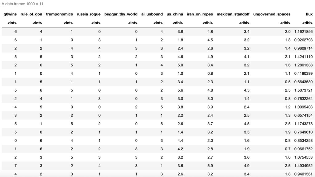
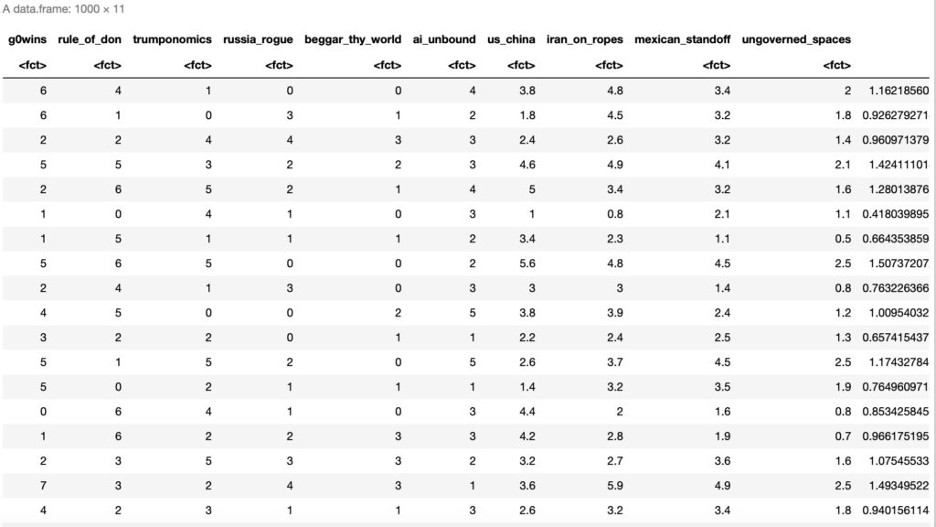
data$flux <- 2 * prob_fluctuation

各係数は実際の観測データを基にしたものではありません。評価用の擬似データです。

生成されたデータは以下のようになります。

pcalg - PC(Peter-Clark)アルゴリズム

　生成したデータセットにPCアルゴリズムを適用します。

#因果探索の実行
suffStat <- list(C = cor(data), n = n)
pc.fit <- pc(suffStat, indepTest = gaussCItest, p = ncol(data), alpha = 0.05)
plot(pc.fit, main="Estimated CPDAG")

　結果をプロットすると以下のDAGが出力されます。

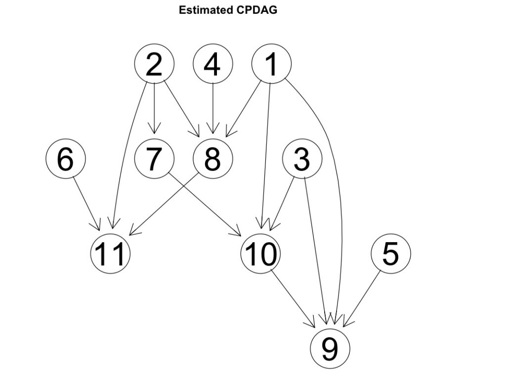
　これはpcalgの出力結果にあるグラフオブジェクトをそのまま表示したものです。

　Rにはigraphライブラリというベイジアンネットワークの描画ツールがあります。これを用いてigraphオブジェクトへの変換関数を作り、見やすいDAGに変換します。表示はigraphライブラリを用いた関数の実装で調整することができます。以下に一例を示します。

#pcalgのオブジェクトをigraphのオブジェクトに変換します。
plot_graph(pc.fit@graph)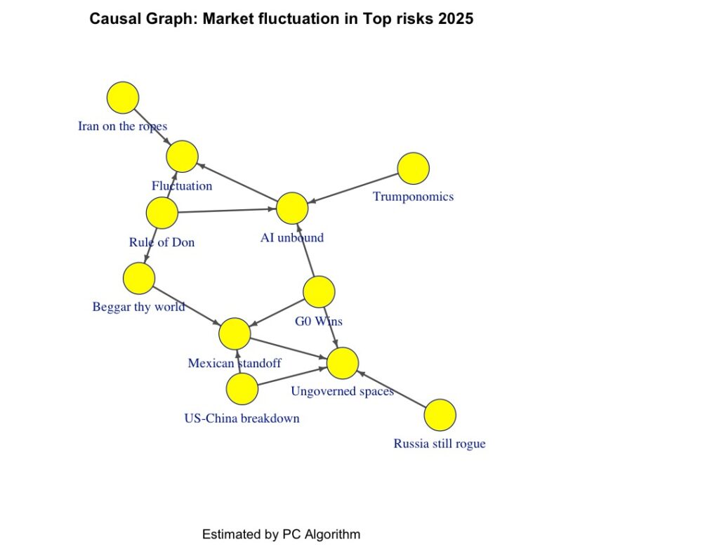

pcアルゴリズムの計算結果の出力は次のようになります。

summary(pc.fit)

Object of class 'pcAlgo', from Call:
pc(suffStat = suffStat, indepTest = gaussCItest, alpha = 0.05, 
    p = ncol(data))

Nmb. edgetests during skeleton estimation:
===========================================
Max. order of algorithm:  3 
Number of edgetests from m = 0 up to m = 3 :  82 226 189 12

Graphical properties of skeleton:
=================================
Max. number of neighbours:  3 at node(s) 1 2 
Avg. number of neighbours:  1.272727 

Adjacency Matrix G:
   1 2 3 4 5 6 7 8 9 10 11
1  . . . . . . . 1 1  1  .
2  . . . . . . 1 1 .  .  1
3  . . . . . . . . 1  1  .
4  . . . . . . . 1 .  .  .
5  . . . . . . . . 1  .  .
6  . . . . . . . . .  .  1
7  . . . . . . . . .  1  .
8  . . . . . . . . .  .  1
9  . . . . . . . . .  .  .
10 . . . . . . . . 1  .  .
11 . . . . . . . . .  .  .

PCアルゴリズム

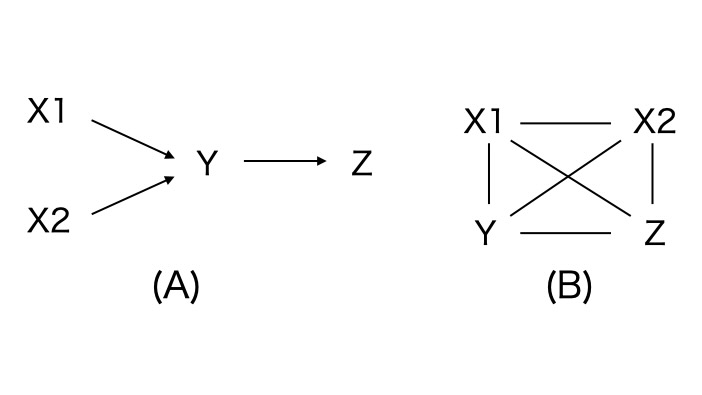
（A）基の真の因果グラフ、（B） PCアルゴリズムは、全てノードが無方向に接続されたグラフから始めます。

（C） X1⊥X2 (X1とX2が独立)のため、X1-X2の接続線が削除されます。（D） X1⊥Z | Y (X1とZがYの条件で独立), X2⊥Z | Y （X2とZがYの条件で独立）のため　X1 - ZとX2 - Zの接続線が削除されます。

　変数のサブセットの条件独立性をチェックを続けます。例えば、YとZは、X1またはX2の条件で独立ではありません。

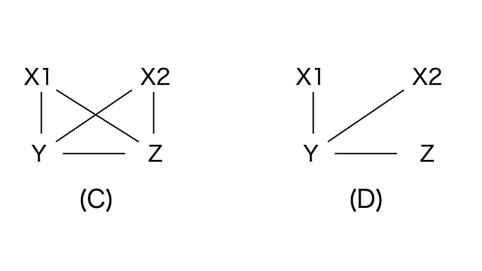
　３変数(A,B,C)の各変数について、AとBが隣接し、BとCが隣接し、AとCが隣接してない場合、もし、BがAとCが独立している条件に無関係ならば、A - B - Cの方向は A → B ← Cになります。このような三つのノードの関係を、v-構造（v-structure）と呼びます。

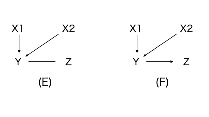
（E）　v-構造が見つかったことからX1,X2の方向はYに向かいます。X1とX2の接続線の削除でYは条件にならないため、X1 - Y - X2の関係は、X1 → Y ← X2です。

　A→ B - Cのような３変数に対して、AとCが隣接していない、B - Cの接続の方向は、B → C 。これを方向の伝播(orientation propagation)と呼びます。

（F） X2 → Y - Zの関係は　X2 → Y → Zのように方向づけられます。

　こうして元の真の構造が探索できました。

(1) P. Spirtes, C. Glymour and R. Scheines (2000). Causation, Prediction, and Search, 2nd edition. The MIT Press.

FCI (Fast Causal Inference) アルゴリズム

　FCIは知られていない交絡因子の探索も実行します。pcalgはFCI,FCI plusというアルゴリズムも提供しています。

fci.fit <- fci(suffStat, indepTest = gaussCItest, p = ncol(data), alpha = 0.9)

Warning message in sqrt(PM[1, 1] * PM[2, 2]):
“計算結果が NaN になりました”

　PCと異なり、graphオブジェクトは出力しません。結果を表示してみます。

summary(fci.fit)

Object of class 'fciAlgo', from Call:
fci(suffStat = suffStat, indepTest = gaussCItest, alpha = 0.9, 
    p = ncol(data))

Nmb. edgetests during skeleton estimation:
===========================================
Max. order of algorithm:  6 
Number of edgetests from m = 0 up to m = 6 :  110 851 1708 1049 253 42 0

Add. nmb. edgetests when using PDSEP:
=====================================
Max. order of algorithm:  9 
Number of edgetests from m = 0 up to m = 9 :  0 156 714 1197 1326 955 588 241 54 6

Size distribution of SEPSET:
   1    2    3    4    5    7 <NA> 
  11   12   25   13    3    2   55 

Size distribution of PDSEP:
 0 10 
 1 10 

Adjacency Matrix G:
G[i,j] = 1/2/3 if edge mark of edge i-j at j is circle/head/tail.

   1 2 3 4 5 6 7 8 9 10 11
1  . . . . . . . . .  2  .
2  . . . . . . 2 . .  .  .
3  . . . . . . . . .  .  .
4  . . . . . . . . .  .  .
5  . . . . . . . . .  .  .
6  . . . . . . . . .  .  .
7  . 1 . . . . . . .  2  .
8  . . . . . . . . .  .  .
9  . . . . . . . . .  .  .
10 1 . . . . . 2 . .  .  .
11 . . . . . . . . .  .  .

デフォルトの表示で結果をplotします。

plot(fci.fit)

fciの計算中に自乗根で計算結果がNaNになっているため、DAGは①、⑦、⑩の関係以外、正しく表示されていません。

(2) Spirtes, P., Meek, C., & Richardson, T. (1995, August). Causal inference in the presence of latent variables and selection bias. In Proceedings of the Eleventh conference on Uncertainty in artificial intelligence (pp. 499-506).
(3) D. Colombo and M. H Maathuis. Order-independent constraint-based causal structure learning.

FCI Plusアルゴリズム

fciPlus.fit <- fciPlus(suffStat, indepTest = gaussCItest, p = ncol(data), alpha = 0.9)

結果を表示します。

 4 *-> 2 <-* 7 
Sxz= and Szx= 3 

 7 *-> 2 <-* 4 
Sxz= 3 and Szx= 

 2 *-> 4 <-* 8 
Sxz= 1 3 7 and Szx= 

 2 *-> 4 <-* 11 
Sxz= 1 3 7 and Szx= 

 8 *-> 4 <-* 2 
Sxz= and Szx= 1 3 7 

 11 *-> 4 <-* 2 
Sxz= and Szx= 1 3 7 

 2 *-> 7 <-* 9 
Sxz= and Szx= 5 10 

 2 *-> 7 <-* 10 
Sxz= and Szx= 5 9 

 9 *-> 7 <-* 2 
Sxz= 5 10 and Szx= 

 10 *-> 7 <-* 2 
Sxz= 5 9 and Szx= 

 4 *-> 8 <-* 9 
Sxz= 1 3 5 10 and Szx= 

 9 *-> 8 <-* 4 
Sxz= and Szx= 1 3 5 10 

 1 *-> 9 <-* 5 
Sxz= and Szx= 3 10 

 1 *-> 9 <-* 8 
Sxz= 2 3 7 and Szx= 

 3 *-> 9 <-* 5 
Sxz= and Szx= 1 10 

 3 *-> 9 <-* 7 
Sxz= and Szx= 1 10 

 3 *-> 9 <-* 8 
Sxz= 1 2 4 and Szx= 

 5 *-> 9 <-* 1 
Sxz= 3 10 and Szx= 

 5 *-> 9 <-* 3 
Sxz= 1 10 and Szx= 

 5 *-> 9 <-* 7 
Sxz= and Szx= 1 

 5 *-> 9 <-* 8 
Sxz= 1 2 4 and Szx= 

 5 *-> 9 <-* 10 
Sxz= 1 3 and Szx= 

 7 *-> 9 <-* 3 
Sxz= 1 10 and Szx= 

 7 *-> 9 <-* 5 
Sxz= 1 and Szx= 

 7 *-> 9 <-* 8 
Sxz= 1 2 3 and Szx= 

 8 *-> 9 <-* 1 
Sxz= and Szx= 2 3 7 

 8 *-> 9 <-* 3 
Sxz= and Szx= 1 2 4 

 8 *-> 9 <-* 5 
Sxz= and Szx= 1 2 4 

 8 *-> 9 <-* 7 
Sxz= and Szx= 1 2 3 

 8 *-> 9 <-* 10 
Sxz= and Szx= 1 2 7 

 10 *-> 9 <-* 5 
Sxz= and Szx= 1 3 

 10 *-> 9 <-* 8 
Sxz= 1 2 7 and Szx= 

 1 *-> 10 <-* 7 
Sxz= and Szx= 9 

 7 *-> 10 <-* 1 
Sxz= 9 and Szx= 

 4 *-> 11 <-* 6 
Sxz= and Szx= 5 

 5 *-> 11 <-* 8 
Sxz= 1 2 4 and Szx= 

 6 *-> 11 <-* 4 
Sxz= 5 and Szx= 

 6 *-> 11 <-* 8 
Sxz= and Szx= 7 

 8 *-> 11 <-* 5 
Sxz= and Szx= 1 2 4 

 8 *-> 11 <-* 6 
Sxz= 7 and Szx= 

Rule 1 
Orient: 9 *-> 8 o-* 11 as: 8 -> 11 

Rule 1 
Orient: 7 *-> 10 o-* 3 as: 10 -> 3 

Rule 2 
Orient: 1 -> 10 *-> 3 or 1 *-> 10 -> 3 with 1 *-o 3 as: 1 *-> 3 

Rule 4 
There is a discriminating path between 7 and 3 for 1 ,and 1 is in Sepset of 3 and 7 . Orient: 1 -> 3

　計算結果をplotで表示します。

plot(fciPlus.fit)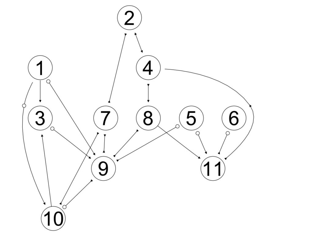

(4) T. Claassen, J. Mooij, and T. Heskes. Learning sparse causal models is not NP-hard. In Proceedings UAI 2013, 2013.

bnlearn

　ベイジアンネットワーク　ライブラリを用いた因果探索の例を示します。

　bnleanの関数の引数に入れるために、すべての変数をfactor (categorical)に変換します。

data[] <- lapply(data, factor)

　data　の構造は以下のようになります。

　このデータセットからベイジアンネットワークの構造を学習します。以下の関数hc()はHill-Climbingを意味し、スコアを基にした学習アルゴリズムです。

bn <- hc(data)

　ここでも、igraphライブラリを使って、表示の様式を変更します。bnleanの出力オブジェクトをigraphのオブジェクトに変換します。

　bnlearnのas.igraphという関数を使います。この関数を使って変換関数を実装し、表示を変更します。以下は一例です。

plot_bn(bn)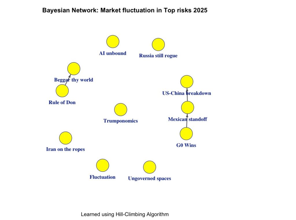

　ベイジアンネットワークの結果を表示します。

print("Summary of the Bayesian Network:")
print(bn)

[1] "Summary of the Bayesian Network:"

  Bayesian network learned via Score-based methods

  model:
   [g0wins][rule_of_don][russia_rogue][beggar_thy_world][ai_unbound]
   [iran_on_ropes][mexican_standoff][flux][us_china|rule_of_don]
   [ungoverned_spaces|g0wins][trumponomics|ungoverned_spaces]
  nodes:                                 11 
  arcs:                                  3 
    undirected arcs:                     0 
    directed arcs:                       3 
  average markov blanket size:           0.55 
  average neighbourhood size:            0.55 
  average branching factor:              0.27 

  learning algorithm:                    Hill-Climbing 
  score:                                 BIC (disc.) 
  penalization coefficient:              3.453878 
  tests used in the learning procedure:  85 
  optimized:                             TRUE

(5) Scutari M (2010). "Learning Bayesian Networks with the bnlearn R Package". Journal of Statistical Software,

MMHC（Max-Min Hill Climbing）アルゴリズム

　MMPC(Max-Min Parents and Children)アルゴリズムとHill-Climbingアルゴリズムを組み合わせたハイブリッドなアルゴリズムです。

# MMHC algorithm (hybrid)
mmhc_dag <- mmhc(data)

　igraphライブラリを使って、表示の様式を変更します。bnleanの出力オブジェクトをigraphのオブジェクトに変換し、DAGの表示を変更します。

plot_mmhc(mmhc_dag, title = "MMHC Algorithm")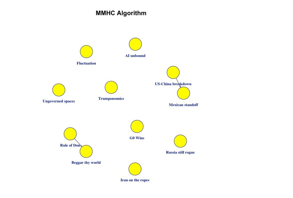

(6) Tsamardinos I, Brown LE, Aliferis CF (2006). "The Max-Min Hill-Climbing Bayesian Network Structure Learning Algorithm". Machine Learning,

Semi-Interleaved HITON-PCアルゴリズム

　変数を減らして、潜在的に多重に関係している複雑なデータセットを使います。PCアルゴリズムを使って、データからDAGの同値類を学習します。

　以下のライブラリを使います。　

　Rgraphviz パッケージがインストールされていない場合、現在、CRANのレポジトリからは削除されているので、パッケージのインストール項に解説しているように、Bioconductorからインストールしてください。

library(bnlearn)
library(pcalg)
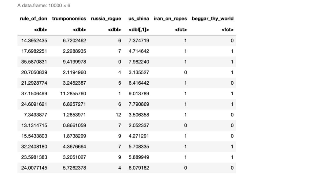
library(Rgraphviz)

　以下の変数名で擬似データを生成します。

rule_of_don
trumponomics
russia_rogue
us_china
iran_on_ropes
beggar_thy_world

set.seed(123)
n <- 10000

data <- data.frame(
  rule_of_don = rnorm(n, mean = 20, sd = 10)
)

data$trumponomics <- exp(0.05 * data$rule_of_don + rnorm(n, 0, 0.5))
data$russia_rogue <- .....
data$us_china <- ......
....

　生成したデータは以下のようになります。

変数の相関関係を調べます。

data$russia_rogue <- as.numeric(data$russia_rogue)
cor_matrix <- cor(data[sapply(data, is.numeric)])
print("Correlation matrix of numeric variables:")
print(cor_matrix)

[1] "Correlation matrix of numeric variables:"
             rule_of_don trumponomics russia_rogue   us_china
rule_of_don    1.0000000    0.6187939   -0.5854584  0.6299120
trumponomics   0.6187939    1.0000000   -0.3632835  0.7777751
russia_rogue  -0.5854584   -0.3632835    1.0000000 -0.3773608
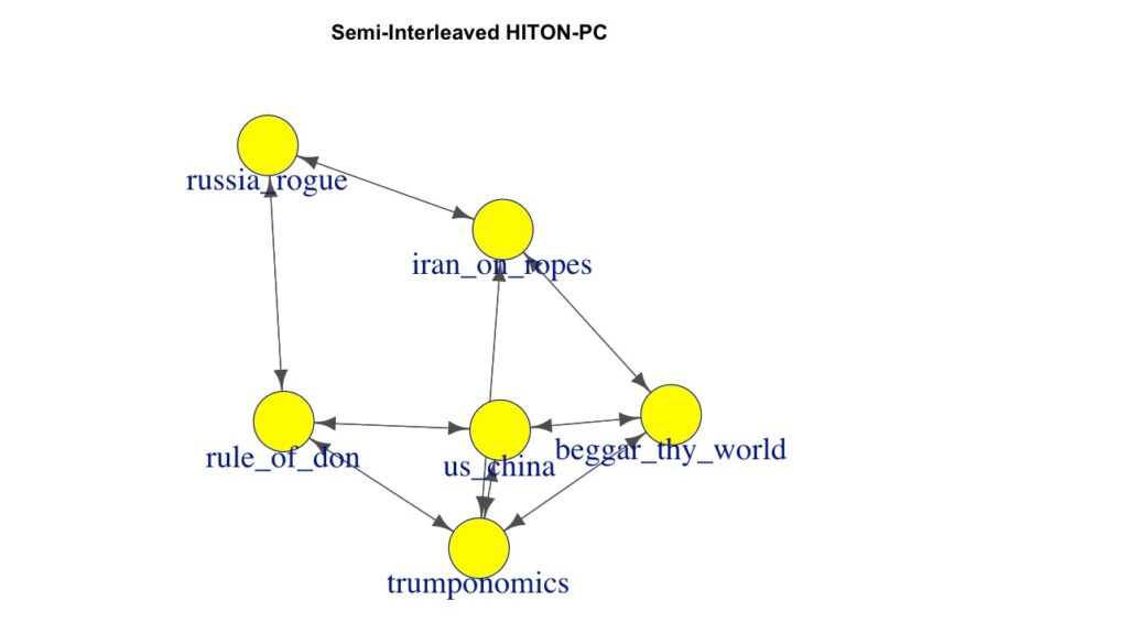
us_china       0.6299120    0.7777751   -0.3773608  1.0000000

　Semi-Interleaved HITON-PCアルゴリズムを使って、ネットワークの構造を学習します。

print("Learning network structure using Semi-Interleaved HITON-PC:")
si_hiton_pc_result <- si.hiton.pc(data)
print(arcs(si_hiton_pc_result))

[1] "Learning network structure using Semi-Interleaved HITON-PC:"
      from               to                
 [1,] "rule_of_don"      "trumponomics"    
 [2,] "rule_of_don"      "russia_rogue"    
 [3,] "rule_of_don"      "us_china"        
 [4,] "trumponomics"     "rule_of_don"     
 [5,] "trumponomics"     "us_china"        
 [6,] "trumponomics"     "beggar_thy_world"
 [7,] "trumponomics"     "iran_on_ropes"   
 [8,] "russia_rogue"     "rule_of_don"     
 [9,] "russia_rogue"     "iran_on_ropes"   
[10,] "us_china"         "rule_of_don"     
[11,] "us_china"         "trumponomics"    
[12,] "us_china"         "beggar_thy_world"
[13,] "iran_on_ropes"    "russia_rogue"    
[14,] "iran_on_ropes"    "trumponomics"    
[15,] "iran_on_ropes"    "beggar_thy_world"
[16,] "beggar_thy_world" "trumponomics"    
[17,] "beggar_thy_world" "us_china"        
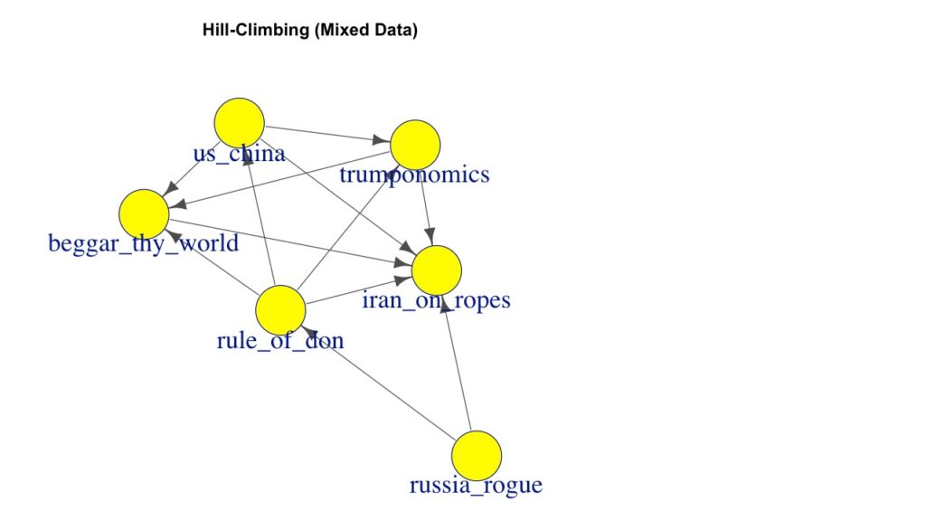
[18,] "beggar_thy_world" "iran_on_ropes"

　同様にスコアを基にした方法でネットワークの構造を学習します。

　Hill-Climbing アルゴリズムがスコア関数を最大化するネットワークの構造を探します。

print("Learning network structure using original data:")
score_hc_result <- hc(data)
print(arcs(score_hc_result))

[1] "Learning network structure using original data:"
      from               to                
 [1,] "trumponomics"     "us_china"        
 [2,] "us_china"         "rule_of_don"     
 [3,] "rule_of_don"      "russia_rogue"    
 [4,] "beggar_thy_world" "trumponomics"    
 [5,] "beggar_thy_world" "us_china"        
 [6,] "trumponomics"     "rule_of_don"     
 [7,] "iran_on_ropes"    "russia_rogue"    
 [8,] "iran_on_ropes"    "trumponomics"    
 [9,] "iran_on_ropes"    "us_china"        
[10,] "iran_on_ropes"    "rule_of_don"     
[11,] "beggar_thy_world" "rule_of_don"     
[12,] "iran_on_ropes"    "beggar_thy_world"

　igraphの形式に変換した、それぞれのDAGを表示します。

　Semi-Interleaved HITON-PCアルゴリズム

スコアを基にしたHill-Climbアルゴリズム

(7) Aliferis FC, Statnikov A, Tsamardinos I, Subramani M, Koutsoukos XD (2010). "Local Causal and Markov Blanket Induction for Causal Discovery and Feature Selection for Classifi-cation Part I: Algorithms and Empirical Evaluation". Journal of Machine Learning Research
(8) Tsamardinos I, Aliferis CF, Statnikov A (2003). "Time and Sample Efficient Discovery of Markov Blankets and Direct Causal Relations". Proceedings of the Ninth ACM SIGKDD International Conference on Knowledge Discovery and Data Mining,

参考資料

(1) P. Spirtes, C. Glymour and R. Scheines (2000). Causation, Prediction, and Search, 2nd edition. The MIT Press.
(2) Spirtes, P., Meek, C., & Richardson, T. (1995, August). Causal inference in the presence of latent variables and selection bias. In Proceedings of the Eleventh conference on Uncertainty in artificial intelligence (pp. 499-506).
(3) D. Colombo and M. H Maathuis. Order-independent constraint-based causal structure learning.
(4) T. Claassen, J. Mooij, and T. Heskes. Learning sparse causal models is not NP-hard. In Proceedings UAI 2013, 2013.
(5) Scutari M (2010). "Learning Bayesian Networks with the bnlearn R Package". Journal of Statistical Software,
(6) Tsamardinos I, Brown LE, Aliferis CF (2006). "The Max-Min Hill-Climbing Bayesian Network Structure Learning Algorithm". Machine Learning,
(7) Aliferis FC, Statnikov A, Tsamardinos I, Subramani M, Koutsoukos XD (2010). "Local Causal and Markov Blanket Induction for Causal Discovery and Feature Selection for Classifi-cation Part I: Algorithms and Empirical Evaluation". Journal of Machine Learning Research
(8) Tsamardinos I, Aliferis CF, Statnikov A (2003). "Time and Sample Efficient Discovery of Markov Blankets and Direct Causal Relations". Proceedings of the Ninth ACM SIGKDD International Conference on Knowledge Discovery and Data Mining,

現代の地政学的な秩序の変化について、同様の指摘をしている識者は少なくありません。例えば、
Peter Zehan, "The End of the World is Just the Beginning: Mapping the Collapse of Globalization"
Victor Shvets, "The Twilight Before the Storm: From the Fractured 1930s to Today's Crisis Culture" ↩︎

グラフィカル・モデルを基にした因果探索

２０２５年の１０大リスク

パッケージのインストール

擬似データの生成

pcalg - PC(Peter-Clark)アルゴリズム

FCI (Fast Causal Inference) アルゴリズム

FCI Plusアルゴリズム

bnlearn

MMHC（Max-Min Hill Climbing）アルゴリズム

Semi-Interleaved HITON-PCアルゴリズム

参考資料

書評：Shocks, Crises, and False Alarms: How to Assess True Macroeconomic Risk

合衆国の新関税の税率と貿易収支

強化学習による因果探索　gCastle因果探索アルゴリズムの検証(3)

CastleBoardの使い方　gCastle因果探索アルゴリズムの検証(2)

マイニング・セクターのリスク許容度、関税の影響　(DoubleMLの推論）